Linear Interpolation Extension Employing Three-Gradient
Speed and Memory Size Optimization
When developing digital signal processor for Deepstomp, we employs a cheap 32-bit processor without floating point unit. Consequently, we have to optimize all computation in fix point math. The most important effect, especially for electric guitar, is distortion effect. It is simulated using sigmoid or sigmoid-like functions such arctan, tanh, or some others. Those functions would consume lot of CPU cycles if implemented using their analytic functions. To solve this, some a linear interpolation extension for one dimensional data is formulated for faster execution.
CMSIS Driver and Table Lookup Solution
Previously, I have tried the simplest approximation using selected range sin function using CMSIS (Cortex Microcontroller Software Interface Standard). The result is still time consuming and eating to much CPU clocks, so we need other solution. The fastest method is table lookup with linear interpolation, but the table could become serious problem. Moreover, some different tables should be used to model various distortion types. The fuzzy type has some extreme non-linearity and I started getting worried about its precision when limiting the table size. After searching for alternative methods, I finally implement my own interpolation method to improve the linear interpolation accuracy.
Linear Interpolation Extension
When talking about two dimensional data and three dimensional data, we can find bilinear and trilinear interpolation extension. But for one dimensional data, I couldn’t find any form of liner extension model. So I think we can improve its accuracy using multiple points of the available data with such extension. In addition, to call it linear, we could do it without introducing the concept of higher order derivatives or polynomial. However, it might be already done by someone else, but it is just beyond my knowledge. So If you know there’s already known method for what I’ll describe in this article, just let me know (in the comment).
Two Point (Linear Interpolation)
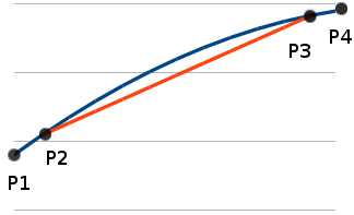
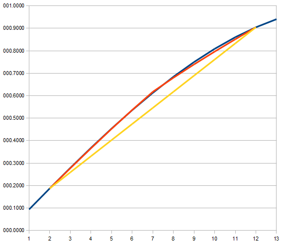
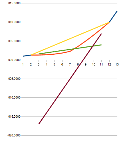
In the Figure 1, the blue line shows the original data between P1 and P4. The other line (red) is the interpolated value between between P2 and P3. The basic linear interpolation uses only P2 and P3 points to calculate all points in between. We can see that the interpolated values has some error distributed along the line. With some error amount proportional (non-linearly) to he distance from the reference point (P2 and P3). We can say that this error is caused by non constant gradient along the line between P1 and P4. Now we can try to correct by the considering the adjacent gradient. Let see how gradient between P1 to P2 and P3 to P4 can be employed. Correction idea for the linear interpolation between P2 to P4 can be shown by plotting the extrapolated values.
Four-Point (3-Gradient) Linear Interpolation Extension
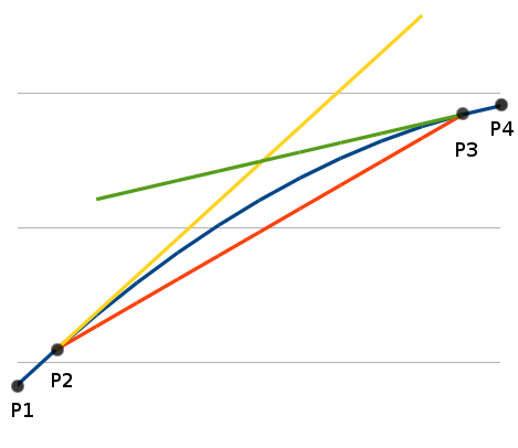
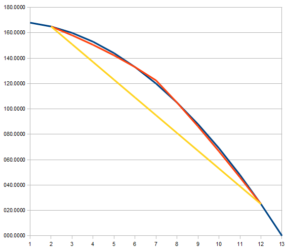
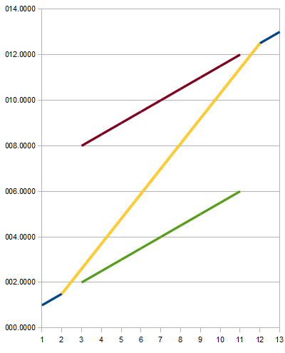
In the Figure 2, the yellow lines shows the extrapolated values using the lower gradient (between P1-P2). While the other line, the green one, is the extrapolated values using the upper gradient (between P3-P4). The interpolated and extrapolated values shows important thing, that the error is zero at the exact reference points. As we can see the error increases as the point goes farther, therefore we can produce a better approximation if we mix the all three lines . It would be made sense if add weights that are inversely proportional to the distance of each reference point.
- The interpolated value (red line) has the zero error at both P2 and P3, so let’s pick the reference point (to compute the weight): the closest one of P2 or P3.
- The lower gradient extrapolated value (yellow line) has zero error at P2, so this is the reference point for it.
- Since the upper gradient extrapolated value (green line) has zero error at P3, so this is the reference point for it.
With P1(x1,y1); P2(x2,y2); P3(x3,y3), and P4(x4,y4) coordinate data, I first formulated the interpolated value at P(x,y) along the lines between P2 and P3 as
- y = f(x,x1,x2,x3,x4,y1,y2,y3,y4);
- = (interpolated * weight + lower_extrapolated * lowerweight + upper_extrapolated * (upperweight)/(totalweight)
- = {{y2 + (x-x2)(y3-y2)/(x3-x2)}*{ 1/(min(x-x2,x3-x))} + {y2 + (x-x2)(y2-y1)/(x2-x1)} * {1/(x-x2)} + {y3 + (x-x3) * (y4-y3)/(x4-x3)}* {1/(x3-x)}}/ {1/(min(x-x2,x3-x)) + 1/(x-x2) + 1/(x3-x)}
Improvement by Weight Modification
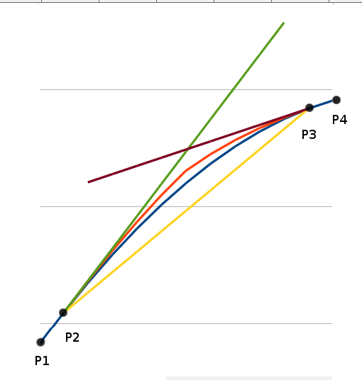
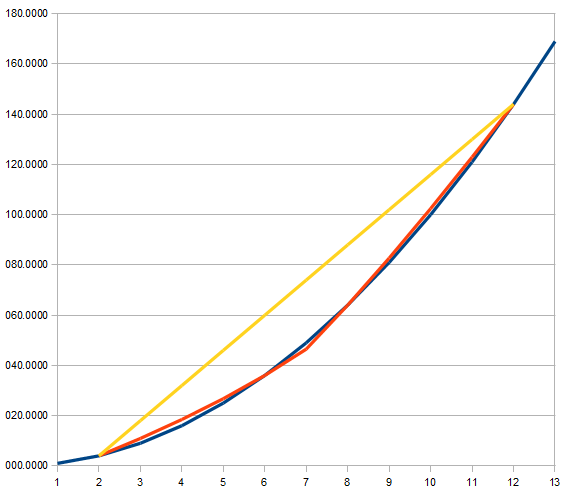
Figure 3 show the interpolated result using the previous formula. It shows the red line as the final result, which is the closest one to the original data (blue line). If we see further detail on the final result, we can see that it still has some distributed errors. By looking at this, I tried to increase the linear weight by doubling it. No the final formula becomes
y = {{y2 + (x-x2)(y3-y2)/(x3-x2)}*{ 2/(min(x-x2,x3-x))}
+ {y2 + (x-x2)(y2-y1)/(x2-x1)} * {1/(x-x2)}
+ {y3 + (x-x3) * (y4-y3)/(x4-x3)}* {1/(x3-x)}}
/ {2/(min(x-x2,x3-x)) + 1/(x-x2) + 1/(x3-x)}
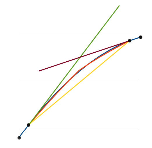
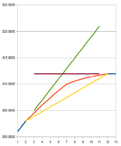
We can see the figure 4 that now the original and the interpolated lines is almost perfectly matched. The following figures (5-10) show several interpolation results using this method for several different 4 point sets.
More Interpolation Examples
Conclusion
We can see the interpolation extension works well in the cases shown in the Figure 5, 6, and 7. Firstly, they have monotonic function and monotonic derivative of the function. Secondly, small change in the gradient from lower to upper data points is shown as their characteristic. The Figure 8 shows more extreme change in the gradient, but the interpolated result seem still acceptable.
When the gradient change is increased to a more extreme level, a case shown in the figure 9 might appear. It is likely not acceptable since we normally assume a smooth transition and monotonic profile int the final result. In the case shown in the Figure 10, we can imagine that the original data has smooth monotonic transition. But the interpolated result is not acceptable because because it has non-monotonic in its derivative. The final interpolated result is unexpected since it shows no improvement from the pure linear interpolation.
In short, this linear interpolation extension will works in some conditions. Firstly, make sure its has monotonic profile on its mapped original data. Secondly, make sure its derivative is monotonic as well. After that, the interpolated result should be acceptable.